61. The Income Fluctuation Problem V: Stochastic Returns on Assets#
GPU
This lecture was built using a machine with access to a GPU.
Google Colab has a free tier with GPUs that you can access as follows:
Click on the “play” icon top right
Select Colab
Set the runtime environment to include a GPU
In addition to what’s in Anaconda, this lecture will need the following libraries:
!pip install quantecon
61.1. Overview#
In this lecture, we continue our study of the income fluctuation problem described in The Income Fluctuation Problem III: The Endogenous Grid Method.
While the interest rate was previously taken to be fixed, we now allow returns on assets to be state-dependent.
This matches the fact that most households with a positive level of assets face some capital income risk.
It has been argued that modeling capital income risk is essential for understanding the joint distribution of income and wealth (see, e.g., [Benhabib et al., 2015] or [Stachurski and Toda, 2019]).
Theoretical properties of the household savings model presented here are analyzed in detail in [Ma et al., 2020].
In terms of computation, we use a combination of time iteration and the endogenous grid method to solve the model quickly and accurately.
We require the following imports:
import matplotlib.pyplot as plt
import numpy as np
from quantecon import MarkovChain
import jax
import jax.numpy as jnp
from jax import vmap
from typing import NamedTuple
61.2. The Model#
In this section we review the household problem and optimality results.
61.2.1. Set Up#
A household chooses a consumption-asset path \(\{(c_t, a_t)\}\) to maximize
subject to
with initial condition \((a_0, Z_0)=(a,z)\) treated as given.
The only difference from The Income Fluctuation Problem IV: Transient Income Shocks is that \(\{R_t\}_{t \geq 1}\), the gross rate of return on wealth, is allowed to be stochastic.
In particular, we assume that
where
\(R\) and \(Y\) are time-invariant nonnegative functions,
the innovation processes \(\{\zeta_t\}\) and \(\{\eta_t\}\) are IID and independent of each other, and
\(\{Z_t\}_{t \geq 0}\) is a Markov chain on a finite set \(\mathsf Z\)
Let \(P\) represent the Markov matrix for the chain \(\{Z_t\}_{t \geq 0}\).
In what follows, \(\mathbb E_z \hat X\) means expectation of next period value \(\hat X\) given current value \(Z = z\).
61.2.2. Assumptions#
We need restrictions to ensure that the objective (61.1) is finite and the solution methods described below converge.
We also need to ensure that the present discounted value of wealth does not grow too quickly.
When \(\{R_t\}\) was constant we required that \(\beta R < 1\).
Since it is now stochastic, we require that
Notice that, when \(\{R_t\}\) takes some constant value \(R\), this reduces to the previous restriction \(\beta R < 1\).
The value \(G_R\) can be thought of as the long run (geometric) average gross rate of return.
More intuition behind (61.4) is provided in [Ma et al., 2020].
Discussion on how to check it is given below.
Finally, we impose some routine technical restrictions on non-financial income.
One relatively simple setting where all these restrictions are satisfied is the IID and CRRA environment of [Benhabib et al., 2015].
61.2.3. Optimality#
Let the class of candidate consumption policies \(\mathscr C\) be defined as in The Income Fluctuation Problem III: The Endogenous Grid Method.
In [Ma et al., 2020] it is shown that, under the stated assumptions,
any \(\sigma \in \mathscr C\) satisfying the Euler equation is an optimal policy and
exactly one such policy exists in \(\mathscr C\).
In the present setting, the Euler equation takes the form
(Intuition and derivation are similar to The Income Fluctuation Problem III: The Endogenous Grid Method.)
We again solve the Euler equation using time iteration, iterating with a Coleman–Reffett operator \(K\) defined to match the Euler equation (61.5).
61.3. Solution Algorithm#
61.3.1. A Time Iteration Operator#
Our definition of the candidate class \(\sigma \in \mathscr C\) of consumption policies is the same as in The Income Fluctuation Problem III: The Endogenous Grid Method.
For fixed \(\sigma \in \mathscr C\) and \((a,z) \in \mathbf S\), the value \(K\sigma(a,z)\) of the function \(K\sigma\) at \((a,z)\) is defined as the \(\xi \in (0,a]\) that solves
The idea behind \(K\) is that, as can be seen from the definitions, \(\sigma \in \mathscr C\) satisfies the Euler equation if and only if \(K\sigma(a, z) = \sigma(a, z)\) for all \((a, z) \in \mathbf S\).
This means that fixed points of \(K\) in \(\mathscr C\) and optimal consumption policies exactly coincide (see [Ma et al., 2020] for more details).
61.3.2. Convergence Properties#
As before, we pair \(\mathscr C\) with the distance
It can be shown that
\((\mathscr C, \rho)\) is a complete metric space,
there exists an integer \(n\) such that \(K^n\) is a contraction mapping on \((\mathscr C, \rho)\), and
The unique fixed point of \(K\) in \(\mathscr C\) is the unique optimal policy in \(\mathscr C\).
We now have a clear path to successfully approximating the optimal policy: choose some \(\sigma \in \mathscr C\) and then iterate with \(K\) until convergence (as measured by the distance \(\rho\)).
61.3.3. Using an Endogenous Grid#
In the study of that model we found that it was possible to further accelerate time iteration via the endogenous grid method.
We will use the same method here.
The methodology is the same as it was for the optimal growth model, with the minor exception that we need to remember that consumption is not always interior.
In particular, optimal consumption can be equal to assets when the level of assets is low.
61.3.3.1. Finding Optimal Consumption#
The endogenous grid method (EGM) calls for us to take a grid of savings values \(s_i\), where each such \(s\) is interpreted as \(s = a - c\).
For the lowest grid point we take \(s_0 = 0\).
For the corresponding \(a_0, c_0\) pair we have \(a_0 = c_0\).
This happens close to the origin, where assets are low and the household consumes all that it can.
Although there are many solutions, the one we take is \(a_0 = c_0 = 0\), which pins down the policy at the origin, aiding interpolation.
For \(s > 0\), we have, by definition, \(c < a\), and hence consumption is interior.
Hence the max component of (61.5) drops out, and we solve for
at each \(s_i\).
61.3.3.2. Iterating#
Once we have the pairs \(\{s_i, c_i\}\), the endogenous asset grid is obtained by \(a_i = c_i + s_i\).
Also, we held \(z \in \mathsf Z\) in the discussion above so we can pair it with \(a_i\).
An approximation of the policy \((a, z) \mapsto \sigma(a, z)\) can be obtained by interpolating \(\{a_i, c_i\}\) at each \(z\).
In what follows, we use linear interpolation.
61.3.4. Testing the Assumptions#
Convergence of time iteration is dependent on the condition \(\beta G_R < 1\) being satisfied.
One can check this using the fact that \(G_R\) is equal to the spectral radius of the matrix \(L\) defined by
This identity is proved in [Ma et al., 2020], where \(\phi\) is the density of the innovation \(\zeta_t\) to returns on assets.
(Remember that \(\mathsf Z\) is a finite set, so this expression defines a matrix.)
Checking the condition is even easier when \(\{R_t\}\) is IID.
In that case, it is clear from the definition of \(G_R\) that \(G_R\) is just \(\mathbb E R_t\).
We test the condition \(\beta \mathbb E R_t < 1\) in the code below.
61.4. Implementation#
Here’s the model as a NamedTuple.
class IFP(NamedTuple):
    """
    A NamedTuple that stores primitives for the income fluctuation
    problem, using JAX.
    """
    γ: float
    β: float
    P: jnp.ndarray
    a_r: float
    b_r: float
    a_y: float
    b_y: float
    s_grid: jnp.ndarray
    η_draws: jnp.ndarray
    ζ_draws: jnp.ndarray


def create_ifp(γ=1.5,
                   β=0.96,
                   P=np.array([(0.9, 0.1),
                               (0.1, 0.9)]),
                   a_r=0.16,
                   b_r=0.0,
                   a_y=0.2,
                   b_y=0.5,
                   shock_draw_size=100,
                   grid_max=100,
                   grid_size=100,
                   seed=1234):
    """
    Create an instance of IFP with the given parameters.
    """
    # Test stability assuming {R_t} is IID and adopts the lognormal
    # specification given below.  The test is then β E R_t < 1.
    ER = np.exp(b_r + a_r**2 / 2)
    assert β * ER < 1, "Stability condition failed."

    # Convert to JAX arrays
    P = jnp.array(P)

    # Generate random draws using JAX
    key = jax.random.PRNGKey(seed)
    key, subkey1, subkey2 = jax.random.split(key, 3)
    η_draws = jax.random.normal(subkey1, (shock_draw_size,))
    ζ_draws = jax.random.normal(subkey2, (shock_draw_size,))
    s_grid = jnp.linspace(0, grid_max, grid_size)

    return IFP(
        γ, β, P, a_r, b_r, a_y, b_y, s_grid, η_draws, ζ_draws
    )


def u_prime(c, γ):
    """Marginal utility"""
    return c**(-γ)

def u_prime_inv(c, γ):
    """Inverse of marginal utility"""
    return c**(-1/γ)

def R(z, ζ, a_r, b_r):
    """Gross return on assets"""
    return jnp.exp(a_r * ζ + b_r)

def Y(z, η, a_y, b_y):
    """Labor income"""
    return jnp.exp(a_y * η + (z * b_y))
Here’s the Coleman-Reffett operator using JAX:
@jax.jit
def K(ae_vals, c_vals, ifp):
    """
    The Coleman--Reffett operator for the income fluctuation problem,
    using the endogenous grid method with JAX.

        * ifp is an instance of IFP
        * ae_vals[i, z] is an asset grid
        * c_vals[i, z] is consumption at ae_vals[i, z]
    """

    # Extract parameters from ifp
    γ, β, P = ifp.γ, ifp.β, ifp.P
    a_r, b_r, a_y, b_y = ifp.a_r, ifp.b_r, ifp.a_y, ifp.b_y
    s_grid, η_draws, ζ_draws = ifp.s_grid, ifp.η_draws, ifp.ζ_draws
    n = len(P)

    # Allocate memory
    c_out = jnp.empty_like(c_vals)

    # Obtain c_i at each s_i, z, store in c_out[i, z], computing
    # the expectation term by Monte Carlo
    def compute_expectation(s, z):
        """Compute expectation for given s and z"""
        def inner_expectation(z_hat):
            # Vectorize over shocks
            def compute_term(η, ζ):
                R_hat = R(z_hat, ζ, a_r, b_r)
                Y_hat = Y(z_hat, η, a_y, b_y)
                a_val = R_hat * s + Y_hat
                # Interpolate consumption
                c_interp = jnp.interp(a_val, ae_vals[:, z_hat], c_vals[:, z_hat])
                U = u_prime(c_interp, γ)
                return R_hat * U

            # Vectorize over all shock combinations
            η_grid, ζ_grid = jnp.meshgrid(η_draws, ζ_draws, indexing='ij')
            terms = vmap(vmap(compute_term))(η_grid, ζ_grid)
            return P[z, z_hat] * jnp.mean(terms)

        # Sum over z_hat states
        Ez = jnp.sum(vmap(inner_expectation)(jnp.arange(n)))
        return u_prime_inv(β * Ez, γ)

    # Vectorize over s_grid and z
    c_out = vmap(vmap(compute_expectation, in_axes=(None, 0)),
                  in_axes=(0, None))(s_grid, jnp.arange(n))

    # Calculate endogenous asset grid
    ae_out = s_grid[:, None] + c_out

    # Fixing a consumption-asset pair at (0, 0) improves interpolation
    c_out = c_out.at[0, :].set(0)
    ae_out = ae_out.at[0, :].set(0)

    return ae_out, c_out
The next function solves for an approximation of the optimal consumption policy via time iteration using JAX:
def solve_model_time_iter(
        model,        # Class with model information
        a_vec,        # Initial condition for assets
        σ_vec,        # Initial condition for consumption
        tol=1e-4,
        max_iter=1000,
        verbose=True,
        print_skip=25
    ):

    # Set up loop
    i = 0
    error = tol + 1

    while i < max_iter and error > tol:
        a_new, σ_new = K(a_vec, σ_vec, model)
        error = jnp.max(jnp.abs(σ_vec - σ_new))
        i += 1
        if verbose and i % print_skip == 0:
            print(f"Error at iteration {i} is {error}.")
        a_vec, σ_vec = a_new, σ_new

    if error > tol:
        print("Failed to converge!")
    elif verbose:
        print(f"\nConverged in {i} iterations.")

    return a_new, σ_new
Now we can create an instance and solve the model using JAX:
ifp = create_ifp()
W1130 23:06:59.736553    2088 cuda_executor.cc:1802] GPU interconnect information not available: INTERNAL: NVML doesn't support extracting fabric info or NVLink is not used by the device.
W1130 23:06:59.740062    2020 cuda_executor.cc:1802] GPU interconnect information not available: INTERNAL: NVML doesn't support extracting fabric info or NVLink is not used by the device.
Set up the initial condition:
# Initial guess of σ = consume all assets
k = len(ifp.s_grid)
n = len(ifp.P)
σ_init = jnp.empty((k, n))
for z in range(n):
    σ_init = σ_init.at[:, z].set(ifp.s_grid)
a_init = σ_init.copy()
Let’s generate an approximation solution with JAX:
a_star, σ_star = solve_model_time_iter(ifp, a_init, σ_init, print_skip=5)
Error at iteration 5 is 5.108221054077148.
Error at iteration 10 is 1.1375703811645508.
Error at iteration 15 is 0.4760274887084961.
Error at iteration 20 is 0.25199270248413086.
Error at iteration 25 is 0.15015077590942383.
Error at iteration 30 is 0.09590339660644531.
Error at iteration 35 is 0.06389141082763672.
Error at iteration 40 is 0.04367399215698242.
Error at iteration 45 is 0.030310630798339844.
Error at iteration 50 is 0.02120828628540039.
Error at iteration 55 is 0.014889717102050781.
Error at iteration 60 is 0.010457038879394531.
Error at iteration 65 is 0.007330417633056641.
Error at iteration 70 is 0.005123615264892578.
Error at iteration 75 is 0.0035686492919921875.
Error at iteration 80 is 0.002475738525390625.
Error at iteration 85 is 0.0017118453979492188.
Error at iteration 90 is 0.0011792182922363281.
Error at iteration 95 is 0.0008096694946289062.
Error at iteration 100 is 0.0005540847778320312.
Error at iteration 105 is 0.00037860870361328125.
Error at iteration 110 is 0.0002579689025878906.
Error at iteration 115 is 0.00017547607421875.
Error at iteration 120 is 0.00011873245239257812.

Converged in 123 iterations.
61.5. Simulation#
Let’s return to the default model and study the stationary distribution of assets.
Our plan is to run a large number of households forward for \(T\) periods and then histogram the cross-sectional distribution of assets.
Set num_households=50_000, T=500.
First we write a function to run a single household forward in time and record the final value of assets.
The function takes a solution pair c_vec and a_vec, understanding them
as representing an optimal policy associated with a given model ifp
@jax.jit
def simulate_household(
        key, a_0, z_idx_0, c_vec, a_vec, ifp, T
    ):
    """
    Simulates a single household for T periods to approximate the stationary
    distribution of assets.

    - key is the state of the random number generator
    - ifp is an instance of IFP
    - c_vec, a_vec are the optimal consumption policy, endogenous grid for ifp

    """
    # Extract parameters from ifp
    γ, β, P, a_r, b_r, a_y, b_y, s_grid, η_draws, ζ_draws = ifp
    n_z = len(P)

    # Create interpolation function for consumption policy
    σ = lambda a, z_idx: jnp.interp(a, a_vec[:, z_idx], c_vec[:, z_idx])

    # Simulate forward T periods
    def update(t, state):
        a, z_idx = state
        # Draw next shock z' from P[z, z']
        current_key = jax.random.fold_in(key, 3*t)
        z_next_idx = jax.random.choice(current_key, n_z, p=P[z_idx]).astype(jnp.int32)
        # Draw η shock for income
        η_key = jax.random.fold_in(key, 3*t + 1)
        η = jax.random.normal(η_key)
        # Draw ζ shock for return
        ζ_key = jax.random.fold_in(key, 3*t + 2)
        ζ = jax.random.normal(ζ_key)
        # Compute stochastic return
        R_next = R(z_next_idx, ζ, a_r, b_r)
        # Compute income
        Y_next = Y(z_next_idx, η, a_y, b_y)
        # Update assets: a' = R' * (a - c) + Y'
        a_next = R_next * (a - σ(a, z_idx)) + Y_next
        # Return updated state
        return a_next, z_next_idx

    initial_state = a_0, z_idx_0
    final_state = jax.lax.fori_loop(0, T, update, initial_state)
    a_final, _ = final_state
    return a_final
Now we write a function to simulate many households in parallel.
def compute_asset_stationary(
        c_vec, a_vec, ifp, num_households=50_000, T=500, seed=1234
    ):
    """
    Simulates num_households households for T periods to approximate
    the stationary distribution of assets.

    Returns the final cross-section of asset holdings.

    - ifp is an instance of IFP
    - c_vec, a_vec are the optimal consumption policy and endogenous grid.

    """
    # Extract parameters from ifp
    γ, β, P, a_r, b_r, a_y, b_y, s_grid, η_draws, ζ_draws = ifp

    # Start with assets = savings_grid_max / 2
    a_0_vector = jnp.full(num_households, s_grid[-1] / 2)
    # Initialize the exogenous state of each household
    z_idx_0_vector = jnp.zeros(num_households).astype(jnp.int32)

    # Vectorize over many households
    key = jax.random.PRNGKey(seed)
    keys = jax.random.split(key, num_households)
    # Vectorize simulate_household in (key, a_0, z_idx_0)
    sim_all_households = jax.vmap(
        simulate_household, in_axes=(0, 0, 0, None, None, None, None)
    )
    assets = sim_all_households(keys, a_0_vector, z_idx_0_vector, c_vec, a_vec, ifp, T)

    return np.array(assets)
We’ll need some inequality measures for visualization, so let’s define them first:
def gini_coefficient(x):
    """
    Compute the Gini coefficient for array x.

    """
    x = jnp.asarray(x)
    n = len(x)
    x_sorted = jnp.sort(x)
    # Compute Gini coefficient
    cumsum = jnp.cumsum(x_sorted)
    a = (2 * jnp.sum((jnp.arange(1, n+1)) * x_sorted)) / (n * cumsum[-1])
    return a - (n + 1) / n


def top_share(
        x: jnp.array,   # array of wealth values
        p: float=0.01   # fraction of top households (default 0.01 for top 1%)
    ):
    """
    Compute the share of total wealth held by the top p fraction of households.

    """
    x = jnp.asarray(x)
    x_sorted = jnp.sort(x)
    # Number of households in top p%
    n_top = int(jnp.ceil(len(x) * p))
    # Wealth held by top p%
    wealth_top = jnp.sum(x_sorted[-n_top:])
    # Total wealth
    wealth_total = jnp.sum(x_sorted)
    return wealth_top / wealth_total
Now we call the function, generate the asset distribution and visualize it:
ifp = create_ifp()
# Extract parameters for initialization
s_grid = ifp.s_grid
n_z = len(ifp.P)
a_init = s_grid[:, None] * jnp.ones(n_z)
c_init = a_init
a_vec, c_vec = solve_model_time_iter(ifp, a_init, c_init)
assets = compute_asset_stationary(c_vec, a_vec, ifp, num_households=200_000)

# Compute Gini coefficient for the plot
gini_plot = gini_coefficient(assets)

# Plot histogram of log wealth
fig, ax = plt.subplots(figsize=(10, 6))
ax.hist(jnp.log(assets), bins=40, alpha=0.5, density=True)
ax.set(xlabel='log assets', ylabel='density', title="Wealth Distribution")
plt.tight_layout()
plt.show()
Error at iteration 25 is 0.15015077590942383.
Error at iteration 50 is 0.02120828628540039.
Error at iteration 75 is 0.0035686492919921875.
Error at iteration 100 is 0.0005540847778320312.

Converged in 123 iterations.
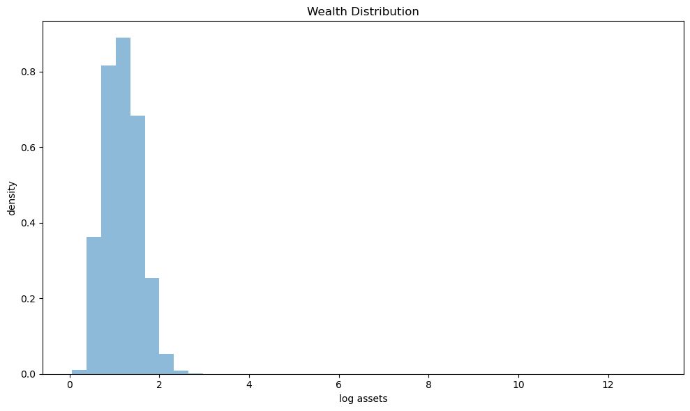
The histogram shows the distribution of log wealth.
Bearing in mind that we are looking at log values, the histogram suggests a long right tail of the distribution.
Below we examine this in more detail.
61.6. Wealth Inequality#
Lets’ look at wealth inequality by computing some standard measures of this phenomenon.
We will also examine how inequality varies with the interest rate.
61.6.1. Measuring Inequality#
Let’s print the Gini coefficient and the top 1% wealth share from our simulation:
gini = gini_coefficient(assets)
top1 = top_share(assets, p=0.01)

print(f"Gini coefficient: {gini:.4f}")
print(f"Top 1% wealth share: {top1:.4f}")
Gini coefficient: 0.7870
Top 1% wealth share: 0.7333
Recent numbers suggest that
the Gini coefficient for wealth in the US is around 0.8
the top 1% wealth share is over 0.3
Our model with stochastic returns generates a Gini coefficient close to the empirical value, demonstrating that capital income risk is an important factor in wealth inequality.
The top 1% wealth share is, however, too large.
Our model needs proper calibration and additional work – we set these tasks aside for now.
61.7. Exercises#
Exercise 61.1
Plot how the Gini coefficient varies with the volatility of returns on assets.
Specifically, compute the Gini coefficient for values of a_r ranging from 0.10 to 0.16 (use at least 5 different values) and plot the results.
What does this tell you about the relationship between capital income risk and wealth inequality?
Solution
We loop over different values of a_r, solve the model for each, simulate the wealth distribution, and compute the Gini coefficient.
# Range of a_r values to explore
a_r_vals = np.linspace(0.10, 0.16, 5)
gini_vals = []

print("Computing Gini coefficients for different return volatilities...\n")

for a_r in a_r_vals:
    print(f"a_r = {a_r:.3f}...", end=" ")

    # Create model with this a_r value
    ifp_temp = create_ifp(a_r=a_r, grid_max=100)

    # Solve the model
    s_grid_temp = ifp_temp.s_grid
    n_z_temp = len(ifp_temp.P)
    a_init_temp = s_grid_temp[:, None] * jnp.ones(n_z_temp)
    c_init_temp = a_init_temp
    a_vec_temp, c_vec_temp = solve_model_time_iter(
        ifp_temp, a_init_temp, c_init_temp, verbose=False
    )

    # Simulate households
    assets_temp = compute_asset_stationary(
        c_vec_temp, a_vec_temp, ifp_temp, num_households=200_000
    )

    # Compute Gini coefficient
    gini_temp = gini_coefficient(assets_temp)
    gini_vals.append(gini_temp)
    print(f"Gini = {gini_temp:.4f}")

# Plot the results
fig, ax = plt.subplots(figsize=(10, 6))
ax.plot(a_r_vals, gini_vals, 'o-', linewidth=2, markersize=8)
ax.set(xlabel='Return volatility (a_r)',
       ylabel='Gini coefficient',
       title='Wealth Inequality vs Return Volatility')
ax.axhline(y=0.8, color='k', linestyle='--', linewidth=1,
           label='Empirical US Gini (~0.8)')
ax.legend()
plt.tight_layout()
plt.show()
Computing Gini coefficients for different return volatilities...

a_r = 0.100...
Gini = 0.1936
a_r = 0.115...
Gini = 0.2004
a_r = 0.130...
Gini = 0.2238
a_r = 0.145...
Gini = 0.3407
a_r = 0.160...
Gini = 0.7870
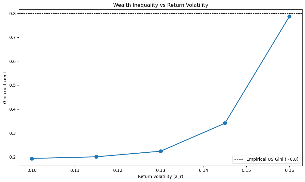
The plot shows that wealth inequality (measured by the Gini coefficient) increases with return volatility.
This demonstrates that capital income risk is a key driver of wealth inequality.
When returns are more volatile, lucky households who experience sequences of high returns accumulate substantially more wealth than unlucky households, leading to greater inequality in the wealth distribution.
Exercise 61.2
Plot how the Gini coefficient varies with the volatility of labor income.
Specifically, compute the Gini coefficient for values of a_y ranging from
0.125 to 0.20 and plot the results. Set a_r=0.10 for this exercise.
What does this tell you about the relationship between labor income risk and wealth inequality? Can we achieve the same rise in inequality by varying labor income volatility as we can by varying return volatility?
Solution
We loop over different values of a_y, solve the model for each, simulate the wealth distribution, and compute the Gini coefficient.
# Range of a_y values to explore
a_y_vals = np.linspace(0.125, 0.20, 5)
gini_vals_y = []

print("Computing Gini coefficients for different labor income volatilities...\n")

for a_y in a_y_vals:
    print(f"a_y = {a_y:.3f}...", end=" ")

    # Create model with this a_y value and a_r=0.10
    ifp_temp = create_ifp(a_y=a_y, a_r=0.10, grid_max=100)

    # Solve the model
    s_grid_temp = ifp_temp.s_grid
    n_z_temp = len(ifp_temp.P)
    a_init_temp = s_grid_temp[:, None] * jnp.ones(n_z_temp)
    c_init_temp = a_init_temp
    a_vec_temp, c_vec_temp = solve_model_time_iter(
        ifp_temp, a_init_temp, c_init_temp, verbose=False
    )

    # Simulate households
    assets_temp = compute_asset_stationary(
        c_vec_temp, a_vec_temp, ifp_temp, num_households=200_000
    )

    # Compute Gini coefficient
    gini_temp = gini_coefficient(assets_temp)
    gini_vals_y.append(gini_temp)
    print(f"Gini = {gini_temp:.4f}")

# Plot the results
fig, ax = plt.subplots(figsize=(10, 6))
ax.plot(a_y_vals, gini_vals_y, 'o-', linewidth=2, markersize=8, color='green')
ax.set(xlabel='Labor income volatility (a_y)',
       ylabel='Gini coefficient',
       title='Wealth Inequality vs Labor Income Volatility')
ax.axhline(y=0.8, color='k', linestyle='--', linewidth=1,
           label='Empirical US Gini (~0.8)')
ax.legend()
plt.tight_layout()
plt.show()
Computing Gini coefficients for different labor income volatilities...

a_y = 0.125...
Gini = 0.1802
a_y = 0.144...
Gini = 0.1833
a_y = 0.163...
Gini = 0.1866
a_y = 0.181...
Gini = 0.1900
a_y = 0.200...
Gini = 0.1936
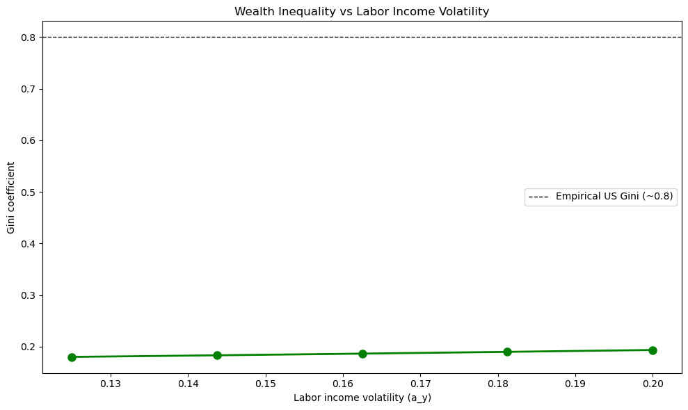
The plot shows that wealth inequality increases with labor income volatility, but the effect is much weaker than the effect of return volatility.
Comparing the two exercises:
When return volatility (
a_r) varies from 0.10 to 0.16, the Gini coefficient rises dramatically from around 0.20 to 0.79When labor income volatility (
a_y) varies from 0.125 to 0.20, a similar amount in percentage terms, the Gini coefficient increases but by a much smaller amount
This suggests that capital income risk is a more important driver of wealth inequality than labor income risk.
The intuition is that wealth accumulation compounds over time: households who experience favorable returns on their assets can reinvest those returns, leading to exponential growth.
In contrast, labor income shocks, while they affect current consumption and savings, do not have the same compounding effect on wealth accumulation.